Learning How to Run with Genetic Algorithms

Overview

When most people think of Deep Reinforcement Learning, they probably think of Q-networks or policy gradients. Both of these methods require you to calculate derivatives and use gradient descent. In this post, we are going to explore a derivative-free method for optimizing a policy network. Specifically, we are going to be using a genetic algorithm on DeepMind’s Control Suite to allow the “cheetah” physical model to learn how to run. You can find the complete code on my github repo.

Genetic Algorithm Background

Genetic algorithms (GAs) are inspired by natural selection, as put forth by Charles Darwin. The idea is that over generations, the heritable traits of a population change because of mutation and the concept of survival of the fittest.

Similar to natural selection, GAs iterate over multiple generations to evolve a population. The population in our case is going to consist of a bunch of neural network weights, which define our cheetah agents. You can think of each set of neural network weights as an individual agent in the population - usually called a chromosome or genotype. Chromosomes are usually encoded as binary strings, but since we want to optimize neural networks weights, we will adapt it for continuous numbers. Each neural network weight in our chromosome can be referred to as a gene. After iterating through all the generations, and continually improving the cheetah’s chromosome (its neural network weights), we hope that it learns how to run.

Initialization

To begin the process, we need to initialize our population of agents. We sample the initial neural network weights from a normal distribution with a scaling factor outlined in Glorot and Bengio’s paper:

\[Var[W^i] = \frac{2}{n_i + n_{i+1}}\]

where \(W^i\) refers to the weight matrix in the \(i^\text{th}\) layer, while \(n_i\) and \(n_{i+1}\) refer to the input and output dimensionality of that layer. Below you’ll see python code to implement the population initialization, where scaling_factor is a vector of variances calculated according to the equation above:

  population = np.random.multivariate_normal(mean = [0]*scaling_factor.shape[0],
                                             cov = np.diag(scaling_factor),
                                             size = population_size)  

Selection

Now that we have a population, we can have the agents within the population compete against each other! The agents that are the most “fit” have the highest probability of passing their genes onto the next generation. We will define fitness as the cumulative reward of our agent over the span of an episode. As you might have guessed by the way we defined it, fitness refers to how good an agent is at performing the task we want it to learn. Those that are better at performing the task will have a better chance of being selected as parents to breed a new generation. There are two primary methods for parent selection - Roulette and Tournament.

The roulette method selects parents with a probability proportional to their fitness score. This is why it is also called Fitness Proportionate Selection.

  # Roulette Wheel Selection
  position = []
  for i in range(2):
      random_number = np.random.uniform(low = 0, high = scores_cumulsum[-1])
      position.append(next(x[0] for x in enumerate(scores_cumulsum) if x[1] > random_number))

  parent_1 = population[population_index_sorted[position[0]]]
  parent_2 = population[population_index_sorted[position[1]]]

The tournament method runs two tournaments in parallel with different subsets of the total population. The competitors for each tournament are chosen at random. The winners from each tournament are selected as the parents to breed the next generation.

  # Tournament Selection
  k = population_size // 2
  tournament_population = np.zeros((k, 2))
  total_competitors = np.random.choice(np.arange(population_size), k * 2, replace = False)
  tournament_population[:,0] = competition_scores[total_competitors[:k]]
  tournament_population[:,1] = competition_scores[total_competitors[k:]]

  parent_indexes = total_competitors[np.argmax(tournament_population, axis = 0) + np.array([0,k])]
  parent_1 = population[parent_indexes[0],]
  parent_2 = population[parent_indexes[1],]

Elitism

One thing we can do to improve performance in our algorithm is introduce the concept of elitism. This refers to the act of carrying over the most fit agents to the next generation without altering their chromosomes through crossover or mutation (which we will explore very soon). We do this because we always want to preserve the best agents from one generation to the next; it is not guaranteed that any of the children will be more fit than their parents.

Crossover

Now that we know how to select the parents from the population, let’s talk breeding! Crossover, also called recombination, takes the chromosomes of two parents and combines them to form children in the next generation. Here are a few ways you can combine two chromosomes:

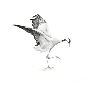
The first and easiest way is to perform One Point crossover. You randomly select a partition in the chromosome, as indicated by the red line below. The child gets the left side of the partition from one parent and the right side from the other parent.

  partition = np.random.randint(0, parent_1.shape[0])
  # Select which parent will be the "left side"
  if which_parent == "Parent 1":
      child = parent_1
      child[partition:] = parent_2[partition:]
  elif which_parent == "Parent 2":
      child = parent_2
      child[partition:] = parent_1[partition:]

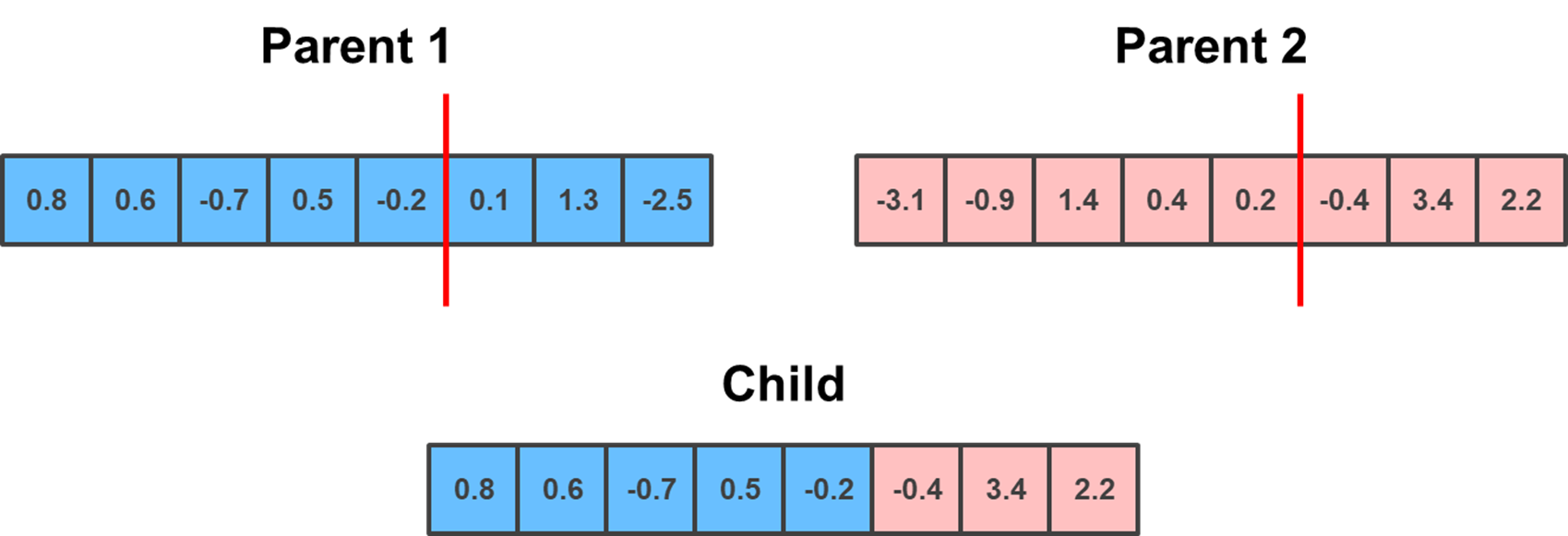
Building on the previous method is Two Point crossover. This is conceptually the same, except you randomly select two points, which serve as a lower and upper bound. The child gets the elements outside of the bounds from one parent, and the elements within the bounds from the other parent.

  lower_limit = np.random.randint(0, parent_1.shape[0]-1)
  upper_limit = np.random.randint(lower_limit+1, parent_1.shape[0])
  # Select which parent will be the "outside bounds"
  if which_parent == "Parent 1":
      child = parent_1
      child[lower_limit:upper_limit+1] = parent_2[lower_limit:upper_limit+1]
  elif which_parent == "Parent 2":
      child = parent_2
      child[lower_limit:upper_limit+1] = parent_1[lower_limit:upper_limit+1]

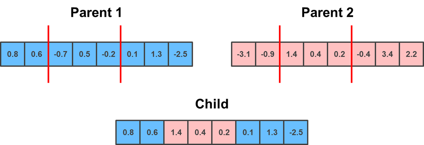
Unlike the previous two methods, which required the swapped genes to be in a sequence, the Uniform crossover does not. Rather, it randomly selects, with a uniform distribution, the indexes to be swapped during crossover.

  random_sequence = np.random.choice(np.arange(parent_1.shape[0]), np.random.randint(1, parent_1.shape[0]), replace = False)
  if which_parent == "Parent 1":
      child = parent_1
      child[np.sort(random_sequence)] = parent_2[np.sort(random_sequence)]
  elif which_parent == "Parent 2":
      child = parent_2
      child[np.sort(random_sequence)] = parent_1[np.sort(random_sequence)]

For the last crossover method, we’ll switch it up a little bit with the Arithmetic crossover. Like the name implies, rather than swapping genes to form a new chromosome, we will do some arithmetics to make a new chromosome. We will perform a simple weighted average on the chromosomes, where the weight is randomly generated.

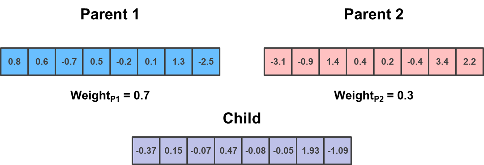
  random_weight = np.random.rand()
  child = parent_1 * random_weight + parent_2 * (1 - random_weight)

Personally, I like using all of the crossover methods, so each time my algorithm performs crossover I randomly select one of the above methods with equal probability.

When setting up a genetic algorithm we define a probability of performing crossover, \(p_\text{cross}\). Thus, with \(1 - p_\text{cross}\) probability, we carry over the parent chromosomes to the next generation without crossover. Since we are going to use elitism in our algorithm, we will probably want to set \(p_\text{cross}\) to be close to 1 because otherwise there is a high probability that we will have duplicate chromosomes in the next generation.

Mutation

After reviewing some of the crossover methods, you might be thinking that we’re just combining genes together without changing their order (with the exception of the arithmetic operator). This means that our chromosomes will be bounded by the initialized values from the first generation, which limits how much our agents can evolve. To ensure this doesn’t happen, we need to maintain genetic diversity - we do this with the mutation operator.

Similar to crossover, there are multiple ways to perform mutation. For my implementation I randomly select a gene with \(p_\text{mutate}\) probability and add gaussian noise to it:

    noise = np.random.standard_normal() * noise_scale
    mutation_position = np.random.randint(0, population.shape[1])
    child[mutation_position] = child[mutation_position] + noise

Even though I remained relatively simple with my implementation, you can get a bit fancier by implementing some of the mutation methods outlined below. The first is the Swap mutation, which selects two random positions in the chromosome and swaps their genes:

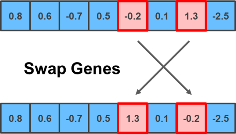
  random_positions = np.random.choice(np.arange(child.shape[0]), 2, replace = False)
  value_1, value_2 = child[random_positions[0]], child[random_positions[1]]
  child[random_positions[0]], child[random_positions[1]] = value_2, value_1

Another method you can implement is the Inversion mutation, which selects two random positions and inverts/reverses the substring of genes between them:

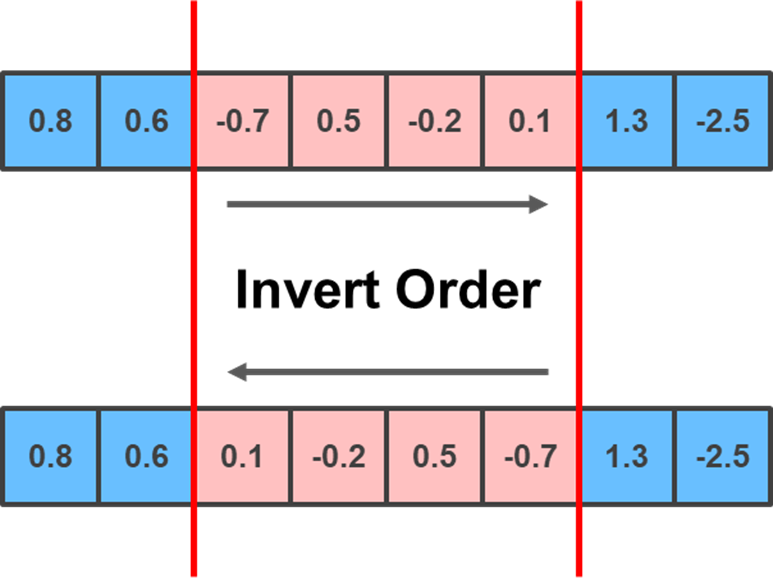
  lower_limit = np.random.randint(0, child.shape[0]-1)
  upper_limit = np.random.randint(lower_limit+1, child.shape[0])
  child[lower_limit:upper_limit+1] = child[lower_limit:upper_limit+1][::-1]

Lastly, you can implement the Scramble mutation, which selects two random positions and scrambles the positions of the genes within them:

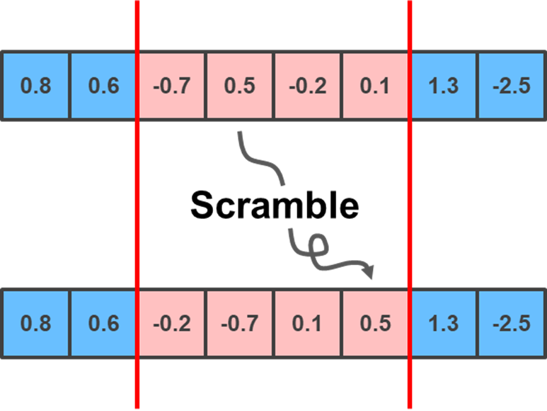
  lower_limit = np.random.randint(0, child.shape[0]-1)
  upper_limit = np.random.randint(lower_limit+1, child.shape[0])
  scrambled_order = np.random.choice(np.arange(lower_limit, upper_limit+1), upper_limit + 1 - lower_limit, replace = False)
  child[lower_limit:upper_limit+1] = child[scrambled_order]

DeepMind’s Control Suite

Great, now that we have all the pieces to make a genetic algorithm, let’s put them together to train the “cheetah” domain from DeepMind’s Control Suite. For those who are not familiar with the library, it is powered by the MuJoCo physics engine and provides you with an environment to train agents on a set of continuous control tasks. For our experiment we want the cheetah to learn how to run.

The thing that I really like about this library is that it has a standardized structure. For example, the library provides you with an observation of the environment and a reward for every action you take. The state observation for our domain task is a combination of the cheetah’s position and velocity. The reward, \(r\), is a function of the forward velocity, \(v\), up to a maximum of \(10 m/s\):

\[r(v) = max(0, min(v/10, 1))\]

We run each episode for 500 frames and calculate the fitness, \(f\), as:

\[f = \sum_{i=1}^{500}r_i\]

At each time step, our agent has to make 6 actions in parallel - the movement of each of its limbs. The action vector for our cheetah has the following property: \(\boldsymbol{a} \in \mathcal{A} \equiv [-1,1]^{6}\). Thus, for our policy, we are going to use a neural network with a 6-dimensional \(\tanh\) output. We flatten all of the neural network weights to a one dimensional array in order to implement the crossover and mutation operators mentioned above. After the child chromosome is created, we reshape the weights to be used in a neural network for the next generation. Overall, we used 1000 generations with a population size of 40 to train our cheetah.

When the training process starts (Generation 1), we see that the cheetah doesn’t know how to move and end up falling backwards:

As training progresses (Generation 250), the cheetah learns how to run forward. However, we see that near the end of the episode it loses control of its stride and falls flat on its face:

At the end of the training process (Generation 1000), we see that the cheetah learns how to run, while also maintaining its center of gravity during large strides:

Awesome, we did it!

Concluding Remarks

In this post we learned how genetic algorithms can be used to optimize parameters of a neural network for a continuous control task. In a future post we will explore an application where we mix genetic algorithms (derivative-free method) and policy gradients (derivative-based method) for better training.