Learning Probability Distributions in Bounded Action Spaces

Overview

In this post we will learn how to apply reinforcement learning in a probabilistic manner. More specifically, we will be looking at some of the difficulties in applying conventional approaches to bounded action spaces, and provide a solution. This blog assumes you have knowledge in deep learning. If not, check out Michael Nielsen’s book - it is very comprehensive and easy to understand.

Reinforcement Learning Background

I am not going to provide a complete background on Reinforcement Learning (RL) because there are already some excellent resources online such as Arthur Juliani’s blogs and David Silver’s lectures. I highly recommend going through both to get a solid understanding of the fundamentals. With that said, I will explain some concepts that are important for this blog post.

At the most basic level, the goal of RL is to learn a mapping from states to actions. To understand what this means, I think it is important to take a step back and understand the RL framework more generally. Cue the overused RL diagram:

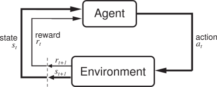
The first thing to notice is that there is a feedback loop between the agent and the environment. For clarity, the agent refers to the AI that we are creating, while the environment refers to the world that the agent has to navigate through. In order to navigate through an environment, the agent has to take actions. The specific actions will depend on the domain - we will describe a few fairly soon. After the agent takes an action, it receives an observation of the environment (the current state) and a reward (assuming we don’t have sparse rewards).

After interacting with the environment for long enough, we hope that our agent learns how to take actions that maximize its cumulative reward over the long-term. It is important to realize that the best action in one state is not necessarily the best action in another state. So going back to our statement about mapping states to actions, this simply means that we want our agent to learn the best actions to take in each environment state. The function that maps states to actions is called a policy and is denoted as \(\pi(a \mid s)\). Usually we read \(\pi(a \mid s)\) as: probability of taking action \(a\), given we are in state \(s\). However, just as a side note, your policy does not have to be defined probabilistically - you can define it deterministically as well.

Now let’s talk a bit about actions an agent can take. The first distinction I would like to make is between discrete actions and continuous actions. When we refer to discrete actions, we simply mean that there is a finite set of possible actions an agent can take. For example, in pong an agent can decide to move up or down. On the other hand, continuous actions have an infinite number of possibilities. An example of a continuous action, although kind of silly, is the hiding position of an agent if it is playing hide and seek.

Given enough time, the agent can theoretically hide anywhere - so the action space is unbounded. In contrast, we can have a continuous action space that is bounded. An example close to my heart is position sizing when trading a financial asset. The bounds are -1 (100% Short) and 1 (100% Long). To map states to that bounded action space, we can use \(\tanh\) in the final layer of a neural network. That seems pretty easy… so why am I writing a blog post about it? Often times we need more than just a deterministic output, especially when the underlying data has a low signal-to-noise ratio. The additional piece of information that we need is uncertainty in our agent’s decision. We will use a Bayesian approach to model a posterior distribution and sample from this distribution to estimate the uncertainty. Don’t worry if that doesn’t completely make sense yet - it will by the end of this post!

Probability Distributions

For a great introduction to Bayesian statistics I suggest reading Will Kurt’s blog - Count Bayesie. It’s awesome.

Distributions can be thought of as representing beliefs about the world. Specifically as it relates to our task at hand, the probability distributions represent our beliefs in how good an action is, given the state. In the financial markets context, where the action space is continuous and bounded between -1 and 1, a mean close to 1 represents a belief that it is a good time to buy that asset, so we should long it. A mean close to -1 represents the opposite, so we should short the asset. Building on this example, if the standard deviation of our distribution is large (small) then our agent is uncertain (certain) in its decision. In other words, if the agent’s policy has a large standard deviation, then it has not developed a strong belief yet.

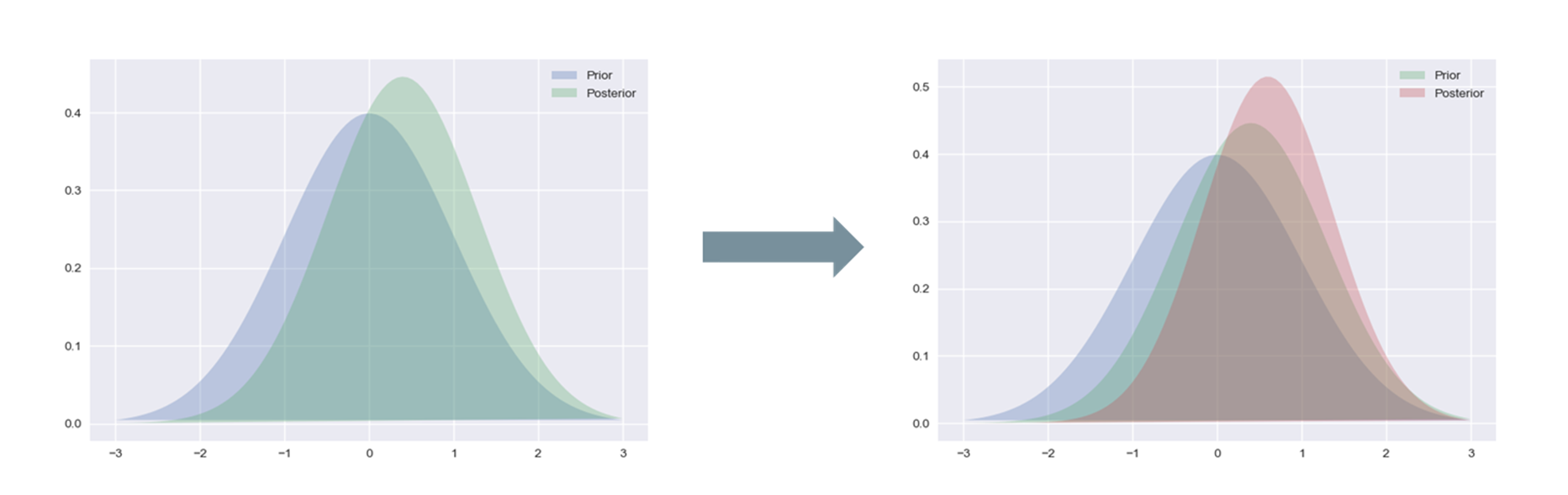
Whenever you hear anyone talking about Bayesian statistics, you always hear the terms “prior” and “posterior”. Simply put, a prior is your belief about the world before receiving new information. However, once you receive new information, then you update your prior distribution to form a posterior distribution. After that, if you receive more information, then your posterior becomes your prior, and the new information gets incorporated to form a new posterior distribution. Essentially, there is this feedback loop of continual learning that happens as more and more new information gets processed by your agent. Below we visually show one iteration of this loop:

Our goal is to learn a good posterior distribution on actions, conditioned on the state that the agent is in. If you are familiar with this paper, then you might be thinking that we can just use Monte Carlo (MC) dropout with a \(\tanh\) output layer. For those who are not familiar with this concept, let me explain. Dropout is a technique that was originally used for neural network regularization. With each pass, it will randomly “drop” neurons from each hidden layer by setting their output to 0. This reduces the output’s dependency on any one particular neuron, which should help generalization. However, researchers at Cambridge found that using dropout during inference can be used to approximate a posterior distribution. This is because each time you pass inputs through the network, a different set of neurons will be dropped, so the output is going to be different for each run - creating a distribution of outputs.

The great thing about this architecture is that you can easily pass gradients through the policy network. The loss function that we are minimizing throughout this blog is \(\mathcal{L} = - r \times \pi(s)\), where \(r\) denotes the reward and \(\pi(s)\) denotes the policy output given the states (i.e. the action). We wanted to demonstrate how the distribution changes in a controlled environment. So we use the same state input throughout all our experiments and continually feed it a positive reward to view the changes during training. Below is the first example using the MC Dropout method and a \(\tanh\) output layer.

I omitted a kernel density estimation (KDE) plot on top of the histogram because as training progressed, the KDE became much more jagged and not representative of the actual probability density function (PDF). I was using sns.kdeplot, if anyone knows how to fix this, please let me know in the comments section!

There are two things that I don’t particularly like about this approach. The first is that it is possible to have multiple peaks in the distribution, as seen when the neural network is first initialized. I realize that as training went on, only one peak emerged. However, the fact that an agent can potentially learn such a distribution (with multiple peaks) makes me uncomfortable. If we go back to our example in the financial markets, an action of -1 will have the exact opposite reward compared to an action of 1 (because it is the other side of the trade), so having peaks at both ends of the spectrum is quite confusing. I would much rather just have one peak near 0 with a large standard deviation if the agent is uncertain which action to take. The second is that it becomes overly optimistic in its decision when compared to a gaussian output (we will see this later), which could possibly indicate that it is understating the uncertainty.

I will digress for a moment to state that a multimodal distribution (a distribution with multiple peaks) is not always bad. For example if you imagine an agent trying to navigate through a room and their policy dictates the angle at which they will move, then there could be two different angles that, while momentarily will send them in different directions, will ultimately lead them to the same end location. However, for this post, we will stick to the example in the financial markets, where a multimodal distribution doesn’t make sense.

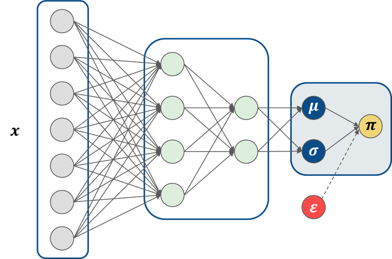
Instead of using MC dropout, we can try using a normal distribution in the output and see if things improve. The architecture of our neural network now becomes:

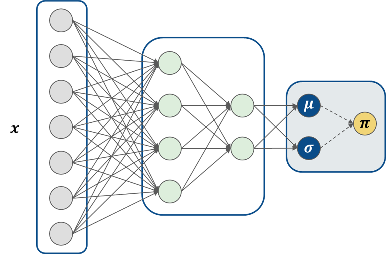
If our neural network parameters are denoted by \(\theta\), then we can define \(\mu_{\theta}\) and \(\sigma_{\theta}\) as outputs of the neural network, such that:

\[\pi \sim \mathcal{N}(\mu_{\theta}(s), \sigma_{\theta}(s))\]

Reparameterization Trick

We want to update the policy network with backpropagation (similar to what we did with the MC dropout architecture), but you’ll notice that we have a bit of a problem - a random variable is now part of the computation graph. This is a problem because backpropagation cannot flow through a random node. However, by using the reparameterization trick, we can move the random node outside of the computation graph and then feed in samples drawn from the distribution as constants. Inference is the exact same, but now our neural network can perform backpropagation.

To do this, we define a random variable \(\varepsilon\), which does not depend on \(\theta\). The new architecture becomes:

\[\varepsilon \sim \mathcal{N}(0,I)\] \[\pi = \mu_{\theta}(s) + \sigma_{\theta}(s) \cdot \varepsilon\]

Python code to take the random variable outside of the computation graph is shown below (I’m only showing the relevant portion of the computation graph):

  import tensorflow as tf

  policy_mu = tf.nn.tanh(tf.matmul(previous_layer, weights_mu) + bias_mu)
  policy_sigma = tf.nn.softplus(tf.matmul(previous_layer, weights_sigma) + bias_sigma)                

  epsilon = tf.random_normal(shape = tf.shape(policy_sigma), mean = 0, stddev = 1, dtype = tf.float32)

  policy = policy_mu + policy_sigma * epsilon

Now to get the neural network to work in a bounded space, we can clip outputs to be between -1 and 1. We simply change the last line of code in our network to:

  policy = tf.clip_by_value(policy_mu + policy_sigma * epsilon, clip_value_min = -1, clip_value_max = 1)

The resulting distribution is shown below:

There is one obvious flaw in this approach - all of the clipped values get a value of either -1 or 1, which creates a very unbalanced distribution. To fix this, we will sample \(\varepsilon\) from a truncated normal distribution.

Truncated Normal Solution

A truncated normal distribution is similar to a normal distribution, in that it is defined by a mean (\(\mu\)) and standard deviation (\(\sigma\)). However, the key distinction is that the distribution’s range is limited to be within a lower and upper bound. Typically the lower bound is denoted by \(a\) and the upper bound is denoted by \(b\), but I’m going to use \(L\) and \(U\) because I think it is easier to follow.

One might think that the bounds we define for the distribution should be the same as the bounds of our policy, but that won’t work if we want to use reparameterization. This is because the bounds apply to \(\varepsilon\) and not \(\pi\). Since we expand \(\varepsilon\) by \(\sigma\) and shift it by \(\mu\), then applying bounds of -1 and 1 will result in a \(\pi\) that extends beyond the bounds. To make this point more clear, let’s say we defined our bounds \(-1 \leq \varepsilon \leq 1\), and \(\mu = 0.5 , \, \sigma = 1\). If we generate a sample \(\varepsilon = 0.9\), then after you apply the transformation \(\mu + \sigma \cdot \varepsilon\), you get \(\pi = 0.5 + 1 \cdot 0.9 = 1.4\), which is beyond the upper bound.

To generate the proper upper and lower bounds, we will use the equations below:

\[L = \frac{-1 - \mu_{\theta}}{\sigma_{\theta}}\] \[U = \frac{1 - \mu_{\theta}}{\sigma_{\theta}}\]

Using our previous example, we find that \(U = 0.5\), which means that the largest \(\varepsilon\) we can sample is 0.5. Plugging this into our reparameterized equation, we see that the largest \(\pi\) we can generate is 1. Similarly, \(L = -1.5\), which means that the lowest \(\pi\) we can generate is -1. Perfect, we figured it out!

Given the PDF for a normal distribution:

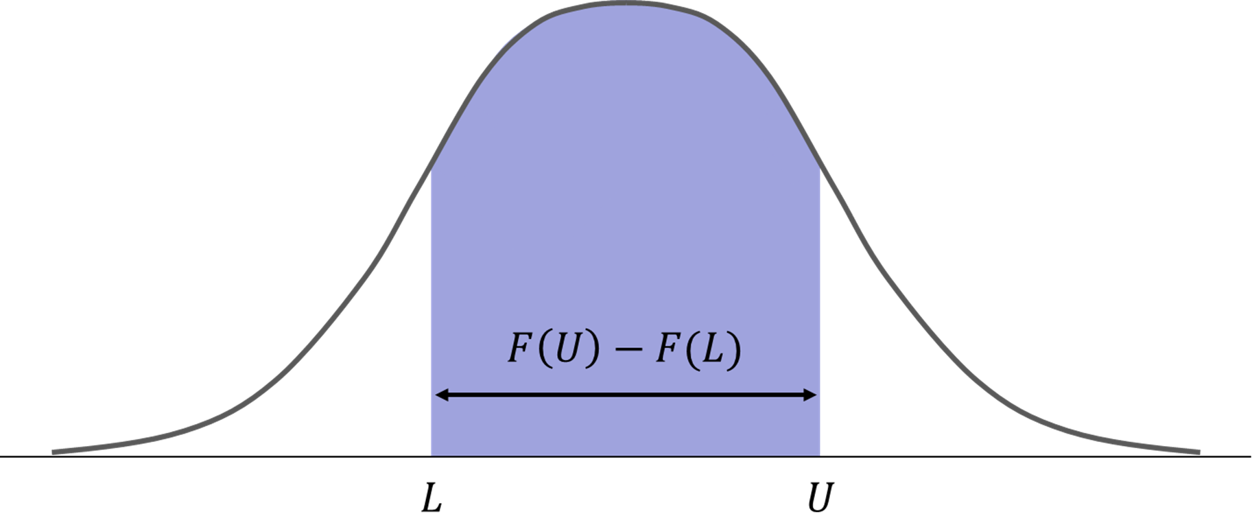
\[p(\varepsilon) = \frac{1}{\sigma\sqrt{2\pi}}e^{-\frac{1}{2}\left(\frac{\varepsilon - \mu}{\sigma}\right)^2}\]

We will let \(F(\varepsilon)\) denote our cumulative distribution function (CDF). Our truncated density now becomes:

\[p(\varepsilon \mid L \leq \varepsilon \leq U) = \frac{p(\varepsilon)}{F(U) - F(L)} \, \, \text{for} \, L \leq \varepsilon \leq U\]

The denominator, \(F(U) - F(L)\), is the normalizing constant that allows the truncated density to integrate to 1. The reason we do this is because, as shown below, we are only sampling from a portion of \(p(\varepsilon)\).

You can import scipy and use the following function to generate samples from a truncated normal distribution:

  import scipy.stats as stats

  mu_dims = 3 # Dimensionality of the Mu generated by the Neural Network

  n_samples = 10000
  sn_mu = 0 # Standard Normal Mu
  sn_sigma = 1 # Standard Normal Sigma

  generator = stats.truncnorm((lower_bound - sn_mu) / sn_sigma, (upper_bound - sn_mu) / sn_sigma, loc = sn_mu, scale = sn_sigma)
  epsilons = generator.rvs([n_samples, mu_dims])

This distribution looks a lot nicer than both of the previous approaches, and has some nice properties:

• It only has one peak at all times
• Outputs do not need to be clipped
• The policy doesn’t look overly optimistic.

Concluding Remarks

In this post, we examined a few approaches to approximating a posterior distribution over our policy. Ultimately, we feel that using a neural network with a truncated normal policy is the best approach out of those examined. We learned how to reparameterize a truncated normal, which allows us to train the policy network using backpropagation.

Acknowledgments

I would like to thank Alek Riley for his feedback on how to improve the clarity of certain explanations.