Accelerated Proximal Policy Optimization

Overview

This post is going to be a little different than the other ones that I’ve made (and probably quite different than most blog posts out there) because I’m not going to be showcasing a finished algorithm. Rather, I’m going to show some of the progress I’ve made in developing a new algorithm that builds off of Proximal Policy Optimization (PPO) and Nesterov’s Accelerated Gradient (NAG). The new algorithm is called Accelerated Proximal Policy Optimization (APPO). The reason I’m making a post about an incomplete algorithm is so other researchers can help accelerate its development. I only ask that you cite this blog post if you use this algorithm in a research paper.

Nesterov’s Accelerated Gradient

We already know how PPO works from my previous blog post, so now the only background information we need is NAG. In this post I will not be explaining how gradient descent works, so for those who are not familiar with gradient descent and want a comprehensive explanation, I highly recommend Sebastian Ruder’s post. I actually used that post to first learn gradient descent a couple years ago.

Below is the update rule for vanilla gradient descent. We have our parameters (weights), \(\theta\), which we update with our gradients \(\nabla_{\theta}J(\theta)\). If you are not familiar with this notation, the \(\nabla_\theta\) refers to a vector of partial derivatives with respect to our parameters (also called the gradient vector). \(J(\theta)\) represents the cost function given our parameters, while \(\eta\) represents our learning rate.

\[\theta = \theta - \eta \nabla_{\theta}J(\theta)\]

The problem with vanilla gradient descent however, is that progress is quite slow during training (shown on the left side of the image below). You will notice a large amount of oscillations across the error surface. To prevent overshooting, we use a small learning rate, which ultimately makes training slow. To help solve this problem, we use the momentum algorithm (shown on the right side of the image below), which is basically just an exponentially weighted average of the gradients.

\[v_t = \gamma v_{t-1} + \eta \nabla_{\theta}J(\theta)\] \[\theta = \theta - v_t\]

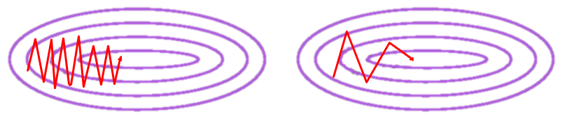
The two new terms introduced in the equations above are \(\gamma\), which is the decay factor, and \(v_t\), which is the exponentially weighted average for the current update. Let’s consider two scenarios to see why momentum helps move our parameters in the right direction faster, while also dampening oscillations. In scenario 1, imagine our previous update \(v_{t-1}\) was a positive number for one of our parameters. Now imagine the current partial derivative for that parameter is also positive. With the momentum update rule, we will be accelerating our parameter update in that direction by adding \(v_{t-1}\) to the already positive partial derivative. The same logic works for negative partial derivatives if \(v_{t-1}\) is negative. In scenario 2, imagine if \(v_{t-1}\) and \(\nabla_{\theta}J(\theta)\) had opposite directions (i.e. one is positive and the other is negative). In that case they will somewhat cancel each other out, which ultimately makes the gradient update smaller (dampening the oscillation).

While this sounds great, there is one pretty obvious flaw in its design - what happens when we have a large momentum term \(v_{t-1}\) and we reached a local minima (i.e. the current gradient is \(\sim 0\))? Well, if we use the momentum update rule, then we will overshoot the local minima because we have to add \(\gamma v_{t-1}\) to the current gradient. To prevent this from happening, we can anticipate the effect of \(\gamma v_{t-1}\) on our parameters and calculate that gradient vector to come up with \(v_t\). So if we used our previous example and assume \(v_{t-1}\) had a large positive value for most of the parameters, then after anticipating what our parameters will be, the gradient vector will consist of mostly negative numbers since we overshot the local minima. Now when we add the two together, they cancel each other out (for the most part). This is know as Nesterov’s Accelerated Gradient and is shown below:

\[v_t = \gamma v_{t-1} + \eta \nabla_{\theta}J(\theta - \gamma v_{t-1})\] \[\theta = \theta - v_t\]

You might be wondering how the concept behind NAG can be used to improve PPO. To understand this, we first need to understand some of the drawbacks of PPO.

Areas of Improvement for PPO

Even though I think PPO is an awesome algorithm, upon examining it more closely I noticed a few things that I would like to improve. I want to change the following aspects of PPO:

1. It is a reactive algorithm and I want to make it a proactive algorithm
2. Using a ratio to measure divergence from the old policy handicaps updates for low probability actions

Before diving into these points, I want to define a word I will be using going forward: training round is defined as the series of updates to our policy network after collecting a certain number of experiences. For example, we can define one training round to be 4 epochs after playing two episodes of a game.

1) Reactive vs Proactive

Clipping only takes effect after the policy gets pushed outside of the range (it also depends on the sign of advantage). As such, it is a reactive algorithm because it only restricts movement once the policy has already moved outside of the specified bounds. This means that PPO does not ensure the new policy is proximal to the old policy because \(r_t(\theta)\) can easily move well below \(1 - \epsilon\) or above \(1 + \epsilon\). As we will see later in this post, by using the accelerated gradient concept behind NAG, we can design a proactive algorithm which anticipates how much the policy will move. We can then use the anticipated move to better control our policy and keep it roughly within the bounds.

2) Ratio vs Absolute Difference

The bounds that we set for the policy in PPO is based off of a ratio, which I do not like. The denominator \(\pi_{\theta_\text{old}}\) matters a lot because if it is too small, then learning is severely impaired. Let’s use an example to show you what I mean. Imagine two scenarios:

1. Low probability action: \(\pi_{\theta_\text{old}}(s_t, a_t) = 2\%\)
2. High probability action: \(\pi_{\theta_\text{old}}(s_t, a_t) = 70\%\)

Now let’s assume that \(\epsilon = 0.2\). This means that we restrict our new policy to be \(1.6\% \leq \pi_\theta \leq 2.4\%\) for the first scenario and \(56\% \leq \pi_\theta \leq 84\%\) for the second scenario. Wait a second… under the first scenario the policy can only move within a range that is \(0.8\%\) wide, while in the second scenario the policy can move within a range that is \(28\%\) wide. If the low probability action should actually have a high probability, then it will take forever to get it to where it should be. However, if we use an absolute difference, then the range in which the new policy can move is the exact same regardless of how small or large the probability of taking an action under our old policy is.

NOTE - There is the obvious exception when the probability of taking an action is near \(0\%\) or \(100\%\). In those cases the lower and upper bound on the new policy is bounded at \(0\%\) and \(100\%\) respectively. However, I don’t consider this a drawback because it is the same when using the ratio.

Initial Attempt to Improve PPO

Let’s deal with the ratio first. In order to get rid of the denominator problem, we define \(\hat{r}_t(\theta)\) as the absolute difference between the new policy and the old policy:

\[\hat{r}_t(\theta) = \left|\pi_\theta(a_t \mid s_t) - \pi_{\theta_\text{old}}(a_t \mid s_t)\right|\]

Next, we need to make the algorithm proactive instead of reactive. To do this, we create an additional neural network that is responsible for telling us how much the policy would change if we implement a policy gradient update. We will denote its parameters as \(\theta_\text{pred}\). At the start of each mini-batch, we reset \(\theta_\text{pred}\) to be equal to \(\theta\). As a result, we can define:

\[\hat{r}_t(\theta_\text{pred}) = \left|\pi_{\theta_\text{pred}}(a_t \mid s_t) - \pi_{\theta_\text{old}}(a_t \mid s_t)\right|\]

Now we can see exactly how much our policy will change if we apply a policy gradient update. In order to constrain the amount our policy can change to be within \(\pi_{\theta_\text{old}}(a_t \mid s_t) \pm \epsilon\), we can calculate the following shrinkage factor:

\[shrinkage = \frac{\epsilon}{\max(\hat{r}_t(\theta_\text{pred}), \epsilon)}\]

I thought that applying this shrinkage factor to the gradients when updating \(\pi_\theta\) will constrain \(\hat{r}_t(\theta) \leq \epsilon\). Boy was I wrong. I was making a linear extrapolation on a function approximation that is non-linear… It was clear that I needed a better way to ensure our policy stays within the specified range per training round.

Current state of APPO

Okay so the shrinkage factor didn’t work, what else can we do? Let’s take a page out of the supervised learning book! After calculating \(\pi_{\theta_\text{pred}}\), we can see if it moves outside of the bounds \(\pi_{\theta_\text{old}}(a_t \mid s_t) \pm \epsilon\). If so, then we can use Mean Squared Error (MSE) as the loss function for those samples and move \(\pi_\theta\) towards the bound that it crossed. On the other hand, if it is within the range, then you can update \(\pi_\theta\) with the regular policy gradient method.

There is one important nuance that we should keep in mind. If we consider a neural network update in isolation, then the method above works great. However, given that we train on multiple mini-batches afterwards, the proceeding change in neural network weights can easily push our policy well beyond our specified range. To prevent this, I found that increasing the number of epochs during training, while also shuffling samples between each epoch significantly reduces the probability of this occurring. I use 10 epochs, but you can probably get away with a smaller number. Empirically, this method has been shown to constrain the new policy to be within the specified bound, with an occasional small deviation outside of the range after each training round.

You will notice that by using the method above, an if statement splits the mini-batch into two smaller batches: one to be trained with MSE and the other to be trained with a policy gradient loss. If you don’t want to split up your mini-batch with an if statement during training, then you can update the whole mini-batch with the following loss function:

\[\mathcal{L} = \frac{1}{n}\sum^n_{i=1}\left(\pi^{(i)}_{\theta} - \text{clip}(\pi^{(i)}_{\theta_\text{pred}}, \pi^{(i)}_{\theta_\text{old}} - \epsilon, \pi^{(i)}_{\theta_\text{old}} + \epsilon)\right)^2\]

This is more computationally expensive because you no longer train a portion of the mini-batch using the policy gradient method (which requires less epochs than the MSE portion). Nonetheless, it is still an option for those who don’t like breaking up the loss function with an if statement.

Concluding Remarks

Results currently look promising, but I don’t think the algorithm is complete. I will continue to work on it and I welcome any feedback!