

Playing Super Mario Bros with Proximal Policy Optimization
Overview
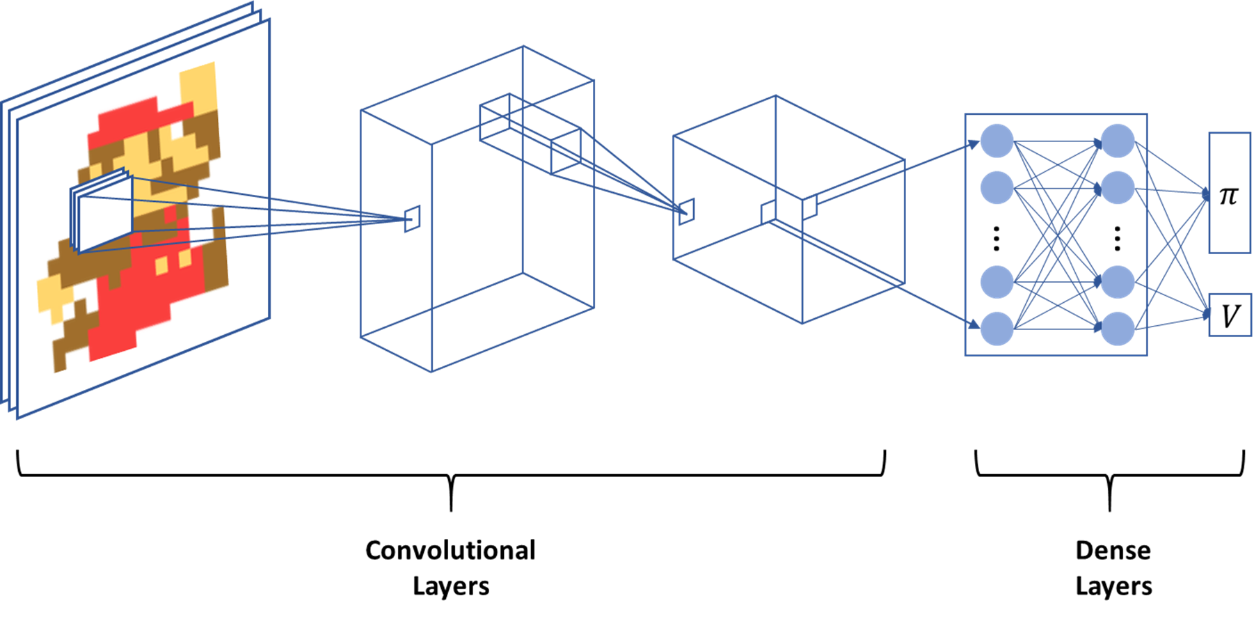
In this post, our AI agent will learn how to play Super Mario Bros by using Proximal Policy Optimization (PPO). We want our agent to learn how to play by only observing the raw game pixels so we use convolutional layers early in the network, followed by dense layers to get our policy and state-value output. The architecture of our model is shown below.
To find the code, please follow this link.
Throughout this post, I’m going to explain each of the model’s components. First we start with the convolutional layers.
Convolutional Neural Network
Convolutional neural networks (CNNs) are widely used in image recognition, and have achieved very impressive results to date. They have their own set of issues, such as the inability to take important spatial hierarchies into account, which capsule networks attempt to address. However, we don’t think that this significantly impacts an agent’s ability to play a video game from raw pixels so convolutional layers will be just fine for our algorithm.
Unfortunately I’m not going to fully explain CNNs because that would take a whole post on its own. Rather, I’m going to explain some of the most important concepts for our model. If you want a more detailed explanation, I highly recommend Chrisopher Olah’s blog - all his posts are incredible. Also Andrew Ng’s course is awesome!
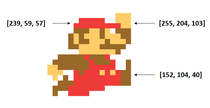
The first thing to understand is that every image is comprised of pixels, and every pixel is represented as a numerical value (or combination of values). The images from the game screen use the RGB color model, which means that for each pixel in the picture, there are going to be 3 numbers associated with it. The numbers correspond to how much red, green, and blue light to add to the image. An example of the RGB codes for the Mario picture are shown below:
Okay great, now what do we do with these pixel values? Convolutional layers are a great way to deal with raw pixel inputs into a neural network. Each convolutional layers consists of multiple filters, which extract important information about an image. You can think of each convolutional layer as a building block for the next. For example, the first layer can put together the pixels to form edges, the second layer can put together the edges to form shapes, the third layer can put the shapes together to form objects, etc.
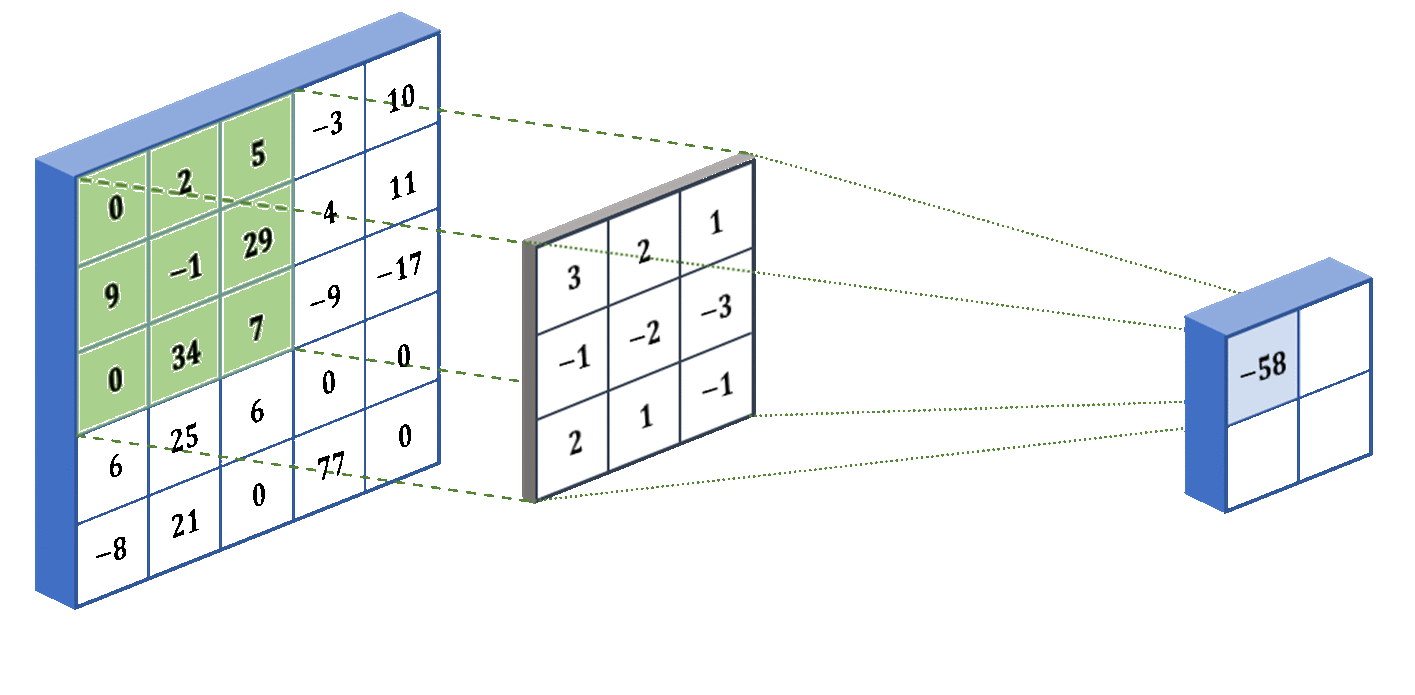
The filters work by performing an operation called convolution, shown in the image below. The operation works by taking the sum of the element-wise product between a portion of the image and the filter (also called a kernel). It focuses on a portion of the image because we need the two matrices to be the same size. In our example, we perform convolution on the bottom-right portion of the image. The filter shown below is specifically designed to detect vertical edges in an image. However, in practice we don’t preset the filter weights to perform a specific task - instead the neural network will learn the weights that it deems the best with backpropagation.
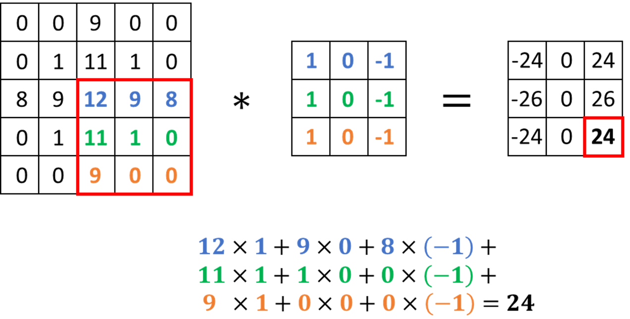
I know I said that the operation being performed above is convolution, but that is not completely true… We’re technically performing cross-correlation, but everyone refers to this operation in the neural network context as convolution. Let me explain why. To actually perform convolution, you need to either flip the source image or the kernel. The reason why we don’t do this for CNNs is because it adds unnecessary complexity. Why is it unnecessary? Because the neural network learns the weights for the kernel anyways, so if you needed to flip the kernel, the CNN will automatically learn the flipped kernel weights, making the actual flipping pointless. Since flipping does not make a difference, cross-correlation is equivalent to convolution in this context.
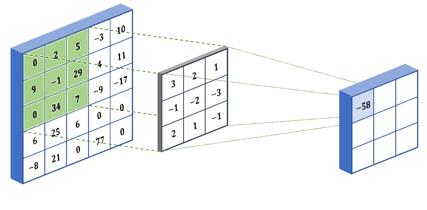
As mentioned before, the kernel is applied to a portion of the image, so we have to slide the kernel over the whole image to account for all the portions. Below we show an example of the filter in action! We used some different numbers - they don’t actually mean anything, I just made them up:
The last concept that I want to introduce for CNNs is stride. The stride determines how many pixels the filter jumps over between convolution operations. For example, in our animation above, the stride was 1 because it moved one pixel at a time. But if we specify a stride of 2, then it will move two pixels at a time (skipping over one pixel). The larger the stride, the smaller the output from the convolutional layer. Below we show what a stride of 2 looks like for the same input and kernel:
Now that we understand how the neural network is able to deal with pixelated inputs, we will move onto the feed-forward (dense) portion of our model - it splits into a value estimation stream and a policy stream. Below we show the implementation of convolutional layers followed by a flattening layer in TensorFlow:
  # Convolutional Layers
  conv1 = tf.layers.conv2d(inputs = inputs, filters = n_filters[0], kernel_size = kernel_size[0],
                           strides = [n_strides[0], n_strides[0]], padding = "valid", activation = tf.nn.elu, trainable = trainable)
  conv2 = tf.layers.conv2d(inputs = conv1, filters = n_filters[1], kernel_size = kernel_size[1],
                           strides = [n_strides[1], n_strides[1]], padding = "valid", activation = tf.nn.elu, trainable = trainable)

  # Flatten the last Convolutional Layer
  first_dimension = round((((image_height - kernel_size[0] + 1) / n_strides[0]) - kernel_size[1] + 1) / n_strides[1])
  second_dimension = round((((image_width - kernel_size[0] + 1) / n_strides[0]) - kernel_size[1] + 1) / n_strides[1])
  dimensionality = first_dimension * second_dimension * n_filters[1]
  conv2_flat = tf.reshape(conv2, [-1, dimensionality])
The Value Function
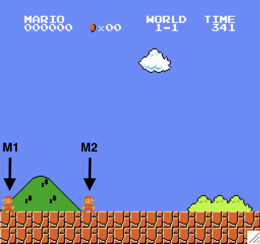
In reinforcement learning, we often care about value functions - specifically, the state-value function \(V(s)\) and the action-value function \(Q(s,a)\). Before diving into some math, I want to explain these concepts intuitively. \(V(s)\) tells us how good it is to be in a particular state. In Super Mario Bros, the goal is to go all the way to the right side of the map, as fast as possible. Thus, we get a positive (negative) reward if we move to the right (left), while getting a negative reward every time the clock ticks. Let’s let M1 and M2 represent two of Mario’s possible positions. If we define \(V(s)\) as the expectation of \(G_t\), which is the cumulative discounted reward from time step \(t\), then we realize that \(V(s_{M2}) > V(s_{M1})\).
If my previous statement did not completely make sense, let’s make it a bit more concrete with some math. Let’s let \(R_t\) represent the reward from time step \(t\). We will define the cumulative discounted reward from time step \(t\) as:
\[G_t = R_{t+1} + \gamma R_{t+2} + \gamma^2 R_{t+3} + \ldots = \sum_{k=0}^{\infty} \gamma^kR_{t+k+1}\]where \(\gamma\) is a discount factor that we apply to future rewards. This is a math trick that makes an infinite sum finite since \(0 \leq \gamma \leq 1\). Although technically if \(\gamma = 1\) then the sum is still infinite because all future rewards have an equal weight. However, we generally use \(\gamma < 1\).
Now that we know how \(G_t\) is defined mathematically, let’s revisit our previous statement: \(V(s_{M2}) > V(s_{M1})\). The farther Mario is from the right, the longer it takes to get to the end of the map. If it takes longer to get to the end of the map, then we have to add up more negative rewards to our cumulative sum (since we get a negative reward every time the clock ticks). Thus, it makes sense that \(V(s_{M2}) > V(s_{M1})\).
Great, now that we have an intuition into how the state-value function works, let’s do some algebra to get a very important equation in reinforcement learning:
\[\begin{align*} V(s) &= \mathbb{E}[\, G_t \, | \, S_t=s \,] \\ &= \mathbb{E}[\, R_{t+1} + \gamma R_{t+2} + \gamma^2 R_{t+3} + \ldots \, | \, S_t=s \,] \\ &= \mathbb{E}[\, R_{t+1} + \gamma (R_{t+2} + \gamma R_{t+3} + \ldots) \, | \, S_t=s \,] \\ &= \mathbb{E}[\, R_{t+1} + \gamma G_{t+1} \, | \, S_t=s \,] \\ &= \mathbb{E}[\, R_{t+1} + \gamma V(S_{t+1}) \, | \, S_t=s \,] \end{align*}\]The equation that we end up with is know as the Bellman equation. If we think about it, it’s actually quite intuitive: the value for being in a particular state is equal to the expected reward we will receive from that state plus the discounted expected value of being in the next state. Let’s break this down a bit more. If the value for being in a state is equal to the sum of discounted future rewards, then \(V(s_{t+1})\) is the sum of discounted rewards after \(t+1\). So if we add \(R_{t+1}\) to \(\gamma V(s_{t+1})\), then we get the sum of discounted rewards after \(t\), which is \(V(s)\).
Alternatively, we can write the Bellman equation as,
\[V(s)=\mathcal{R}_s + \gamma \sum_{s^\prime \in \mathcal{S}} \mathcal{P}_{ss^\prime} V(s^\prime)\]where \(\mathcal{P}_{ss^\prime}\) refers to the probability transition matrix (i.e. the probability of moving from \(s\) to \(s^{\prime}\) for all \(\mathcal{S}\)).
Up until now, we were talking about the state-value function, but what about \(Q(s,a)\)? Most times, people actually care more about \(Q\) than \(V\). The reason is because they want to know how to act in a given state, rather than the value of being in a state. This is exactly what \(Q(s,a)\) helps you determine because it tells you the value for taking a specific action in a given state. Thus, if you calculate the Q-value for all actions you can take (assuming the action space is discrete), then you can choose the action that has the maximum value. The super popular Q-learning algorithm learns the mapping from states to Q-values, so that an agent knows which actions will yield the highest cumulative discounted reward.
Let’s solidify our understanding of state-value and action-value. There is going to be a bit more math in this part, so get ready! First, let’s define a new term: the mapping from states to actions is defined as the policy and is denoted as \(\pi(a \mid s)\). Although policies can be deterministic, we are going to read \(\pi(a \mid s)\) as “the probability of taking an action given the state”. I find that reading equations out loud in plain english helps solidify my understanding, so that’s what I’m going to do for the next few equations.
First we show the value of being in state \(s\) by following policy \(\pi\). It is equal to the sum of Q-values, which correspond to particular actions, multiplied by the probability of taking those actions according to policy \(\pi\).
\[v_{\pi}(s)=\sum_{a \in \mathcal{A}}\pi(a \mid s)q_{\pi}(s,a)\]Let’s break down \(v_{\pi}(s)\) in english:
- In any state, there are multiple actions that we can take
- We take each action according to a probability distribution
- Each action has a different value associated with it
- Thus, the value of being in a state is equal to the weighted average of the action-values, in which the weights are the probabilities of taking each action
Next we show the value of taking action \(a\) in state \(s\) by following policy \(\pi\). It is equal to the expected reward from taking an action plus the discounted expected value of being in the next state.
\[q_{\pi}(s,a)=\mathcal{R}_s^a + \gamma \sum_{s^\prime \in \mathcal{S}}\mathcal{P}_{ss^\prime}^{a}v_{\pi}(s^\prime)\]Let’s break down \(q_{\pi}(s,a)\) in english:
- For any action an agent takes, it receives a reward
- When an agent takes an action, it can end up in a different state
- Image if your action was to move to the right - your agent is now in a new state
- Sometimes environments have randomness embedded in them
- Imagine if you try to move to the right, but wind pushes you back and you end up to the left of your original position
- Thus, by taking an action in a given state, there is a probability that the agent will end up in various new states
- As a result, the value of taking an action in a given state is equal to the immediate reward from taking that action plus the weighted average of state-values for the next state multiplied by a discount factor.
- The weights are the probabilities of ending up in the next states.
The previous two equations shown were half-step lookaheads. To show the full one-step lookaheads, we can plug in the previous equations to obtain the following:
\[v_{\pi}(s)=\sum_{a \in \mathcal{A}}\pi(a \mid s)\left(\mathcal{R}_s^a + \gamma \sum_{s^\prime \in \mathcal{S}}\mathcal{P}_{ss^\prime}^{a}v_{\pi}(s^\prime)\right)\] \[q_{\pi}(s,a)=\mathcal{R}_s^a + \gamma \sum_{s^\prime \in \mathcal{S}}\mathcal{P}_{ss^\prime}^{a}\sum_{a^\prime \in \mathcal{A}}\pi(a^\prime|s^\prime)q_{\pi}(s^\prime,a^\prime)\]If you understood the intuition for the first two equations, then you should have no problem with the two equations above - they are simply an extension using the exact same logic.
Policy Gradient
What if we want to skip the middle part and just learn a mapping from states to actions without estimating the value of taking an action? We can do this with the policy gradient method, in which we explicitly learn \(\pi\)! Well sort of… we will soon see why we will actually need to incorporate the value function, but until then, let’s walk through a simple implementation of a policy gradient. Let’s consider the loss function:
\[\mathcal{L} = r \times \log \pi(s,a)\]We want to maximize \(\mathcal{L}\), which is equivalent to minimizing \(-\mathcal{L}\) (we usually perform gradient descent, so minimizing a loss function is the convention). By minimizing \(-\mathcal{L}\), we ensure that we increase the probability of taking an action that gives us a positive reward, and decrease the probability of taking an action that gives us a negative reward. That seems like a good idea, right? Not really… let’s go through an example to understand why. Imagine there are 3 actions that an agent can take with rewards of \([-1,3,20]\) in particular state. There are two main problems with this approach:
- Credit Assignment Problem
- Multiple “Good” Actions
The credit assignment problem refers to the fact that rewards can be temporally delayed. For example, if an agent takes an action in time step \(t\), the reward might come well after \(t+1\). An example in Super Mario Bros is when our agent has to jump over a tube; multiple frames elapse from the time it presses the jump button to the time it actually makes it over the tube. The number of time steps that can possibly elapse between actions and rewards differ for each situation, so how do we solve this problem? Although this is not a perfect solution, we can use value functions, specifically \(q_{\pi}(s,a)\). Since \(q_{\pi}(s,a)\) sums all future discounted rewards from taking action \(a\) and following policy \(\pi\), our agent can take into account rewards that are temporally delayed. Our loss function now becomes:
\[\mathcal{L} = q_{\pi}(s,a) \times \log \pi(s,a)\]Let’s now assume that \([-1,3,20]\) represents Q-values instead of rewards. We still have an issue because there are multiple actions that have a positive expected value. Imagine if we sample the second action, which has a positive Q-value. Based on our new policy gradient loss function, the parameter update would increase the probability of taking that action since \(q_{\pi}(s,a)\) is positive. But what about action 3? It had a much higher Q-value than action 2, so instead we need a way to tell the model to decease the probability of selecting action 2 and instead select action 3. That is what advantage helps us do.
The Advantage Function
Rather than looking at how good it is to take an action, advantage tells us how good an action is relative to other actions. This subtlety is important because we want to select actions that are better than average, as opposed to any action that has a positive expected value. To do this, we have to strip out the state-value from the action-value to get a pure estimate of how good an action is. We define advantage as:
\[A(s,a) = Q(s,a) - V(s)\]If we assume that our policy follows a uniform distribution (equal probability for each action), then \(V(s) = 7.33\), which means that \(A(s,a) = [-8.3,-4.3,12.7]\). Using our new loss function for policy gradients,
\[\mathcal{L} = A_{\pi}(s,a) \times \log \pi(s,a)\]we see that after selecting action 2, our agent will decrease the probability of selecting that action again in the same state because it has a negative advantage (its value is worse than the average). This is great, it does exactly what we want it to do! However, we don’t know the true advantage function (much like the value functions), so we have to estimate it. Luckily, there are a few ways to do this, but I’m going to focus on one method - using the temporal difference error (\(\delta_{TD}\)) from our value estimation.
Let me back up a little to explain what temporal difference error is. Remember when we saw this somewhat complicated equation earlier:
\[q_{\pi}(s,a)=\mathcal{R}_s^a + \gamma \sum_{s^\prime \in \mathcal{S}}\mathcal{P}_{ss^\prime}^{a}\sum_{a^\prime \in \mathcal{A}}\pi(a^\prime|s^\prime)q_{\pi}(s^\prime,a^\prime)\]Well it turns out that it will come in handy after all! Just a refresher - the equation above considers all possible paths. But what if we just sample one action from our policy and sample the next state from the environment? Well then it becomes:
\[q_{\pi}(s,a) = r + \gamma v_{\pi}(s^{\prime})\]Keep this in mind while I explain \(\delta_{TD}\). As the name implies, temporal difference error refers to the difference between the one-step lookahead and the current estimate. We can calculate \(\delta_{TD}\) for either the state-value or action-value, but in this example we’re using the state-value. When we sample, the one-step lookahead equation for state-value becomes \(v_{\pi}(s) = r + \gamma v_{\pi}(s^{\prime})\). You’ll notice that the left side is a pure estimate, while the right side is a mix of estimation and actual data from the environment. This means that the right side contains more information about the environment than the left! By taking the difference between the two we obtain:
\[\delta_{TD} = r + \gamma v_{\pi}(s^{\prime}) - v_{\pi}(s)\]and by minimizing \(\delta_{TD}^2\), we move our value estimation closer to the actual value function. This is because we are continually moving our estimate closer to a target that contains more data from the actual environment. In addition to using \(\delta_{TD}\) to optimize our value network, it turns out that we can also use it to estimate advantage. Wait, what? How? Let’s bring back \(q_{\pi}(s,a)\):
\[q_{\pi}(s,a) = r + \gamma v_{\pi}(s^{\prime})\]Recall what advantage is defined as:
\[A = Q - V\]Now let’s take a look at \(\delta_{TD}\) again:
\[\delta_{TD} = \underbrace{r + \gamma v_{\pi}(s^{\prime})}_{q_{\pi}(s,a)} - v_{\pi}(s)\]which means that \(\delta_{TD} \approx A\)
Generalized Advantage Estimation
The paper we are referencing in this section was used for continuous control, but it can also be used for a discrete action space, like the one we are working with.
We will denote our advantage estimate as \(\hat{A}_t\). Like any other estimate, \(\hat{A}_t\) is subject to bias (although it has low variance). To get an unbiased estimate, we need to get rid of the value estimate completely and sum all future rewards in an episode. This is known as the Monte Carlo return, and it has high variance. As with most things in machine learning, there is a tradeoff - this one is known as the bias-variance tradeoff in reinforcement learning. Generalized Advantage Estimation (GAE) is a great solution that significantly reduces variance while maintaining a tolerable level of bias. It is parametereized by \(\gamma \in [0,1]\) and \(\lambda \in [0,1]\), where \(\gamma\) is the discount factor mentioned earlier in this blog, and \(\lambda\) is the decay parameter used to take an exponentially weighted average of k-step advantage estimators. It is analogous to Sutton’s TD(\(\lambda\)).
Before we get into some of the math, I want to note that \(\gamma\) and \(\lambda\) serve different purposes. To determine the scale of the value function, we use \(\gamma\). In other words, the value of \(\gamma\) determines how nearsighted (\(\gamma\) near 0) or farsighted (\(\gamma\) near 1) we want our agent to be in its value estimate. No matter how accurate our value function is, if \(\gamma < 1\), we introduce bias into the policy gradient estimate. On the other hand, \(\lambda\) is a decay factor and \(\lambda < 1\) only introduces bias when the value function is inaccurate.
I’m going to spare you the details on the derivation of GAE because I feel like we’ve gone through enough math for one post. However, if you have any questions just let me know in the comments section below and I’ll explain it in-depth. As mentioned before, GAE is defined as the exponentially weighted average of k-step advantage estimators. The equation is shown below:
\[\hat{A}^{GAE(\gamma,\lambda)}_t = \sum^{\infty}_{l=0}(\gamma \lambda)^l\delta_{t+l}\]Below we show an implementation of GAE in python:
  def get_gaes(rewards, state_values, next_state_values, GAMMA, LAMBDA):
      deltas = [r_t + GAMMA * next_v - v for r_t, next_v, v in zip(rewards, next_state_values, state_values)]
      gaes = copy.deepcopy(deltas)
      for t in reversed(range(len(gaes) - 1)):
          gaes[t] = gaes[t] + LAMBDA * GAMMA * gaes[t + 1]
      return gaes, deltas
If you understand the equation above, then you might find this next part pretty cool, otherwise you can just skip over it. There are two special cases of the formula above, when \(\lambda=0\) and \(\lambda=1\):
\[GAE(\gamma,0): \hat{A}_t := \delta_t = r_t + \gamma V(S_{t+1}) - V(S_t)\] \[GAE(\gamma,1): \hat{A}_t := \sum^{\infty}_{l=0}\gamma\delta_{t+l} = \sum^{\infty}_{l=0}\gamma^lr_{t+l} - V(S_t)\]When we have \(0 < \lambda < 1\), our GAE is making a compromise between bias and variance. From now on, our loss function for the policy gradient becomes:
\[\mathcal{L} = \hat{A}^{GAE(\gamma,\lambda)} \times \log \pi(s,a)\]Going forward, when you see \(\hat{A}_t\), we are actually referring to \(\hat{A}^{GAE(\gamma,\lambda)}_t\).
Proximal Policy Optimization
We’re finally done catching up on all the background knowledge - time to learn about Proximal Policy Optimization (PPO)! This algorithm is from OpenAI’s paper, and I highly recommend checking it out to get a more in-depth understanding after reading my blog.
PPO takes inspiration from Trust Region Policy Optimization (TRPO), which maximizes a “surrogate” objective function:
\[L^{CPI}(\theta) = \hat{\mathbb{E}}_t\big[r_t(\theta)\hat{A}_t\big]\]where \(r_t(\theta)\) represents the probability ratio of our current policy versus our old policy:
\[r_t(\theta) = \frac{\pi_{\theta}(a_t \mid s_t)}{\pi_{\theta_\text{old}}(a_t \mid s_t)}\]TRPO also has constraints that I’m not going to get into, but if you’re interested, I highly recommend reading the paper. While TRPO is quite impressive, it is complex and computationally expensive to run. As a result, OpenAI came up with a simpler, more general algorithm that has better sample complexity (empirically). The idea is to limit how much our policy can change during each round of updates by clipping \(r_t(\theta)\) between a range determined by \(\epsilon\):
\[L^{CLIP}(\theta) = \hat{\mathbb{E}}_t\big[\min(r_t(\theta)\hat{A}_t, \text{clip}(r_t(\theta), 1 - \epsilon, 1 + \epsilon)\hat{A}_t)\big]\]The reason we do this is because conventional policy gradient methods are very sensitive to your choice of step size. If the step size is too small then the training progresses too slowly. If the step size is too large then your policy can overshoot the optimal policy during training, making it too noisy. By limiting how much our policy can change, we reduce the sensitivity to the step size. An implementation of \(L^{CLIP}\) in python is shown below:
  with tf.variable_scope('actor_loss'):
      action_probabilities = tf.reduce_sum(policy * tf.one_hot(indices = actions, depth = output_dimension), axis = 1)
      old_action_probabilities = tf.reduce_sum(old_policy * tf.one_hot(indices = actions, depth = output_dimension), axis = 1)

      ratios = tf.exp(tf.log(action_probabilities) - tf.log(old_action_probabilities))
      clipped_ratios = tf.clip_by_value(ratios, clip_value_min = 1 - _clip_value, clip_value_max = 1 + _clip_value)
      clipped_loss = tf.minimum(tf.multiply(GAE, ratios), tf.multiply(GAE, clipped_ratios))
      actor_loss = tf.reduce_mean(clipped_loss)
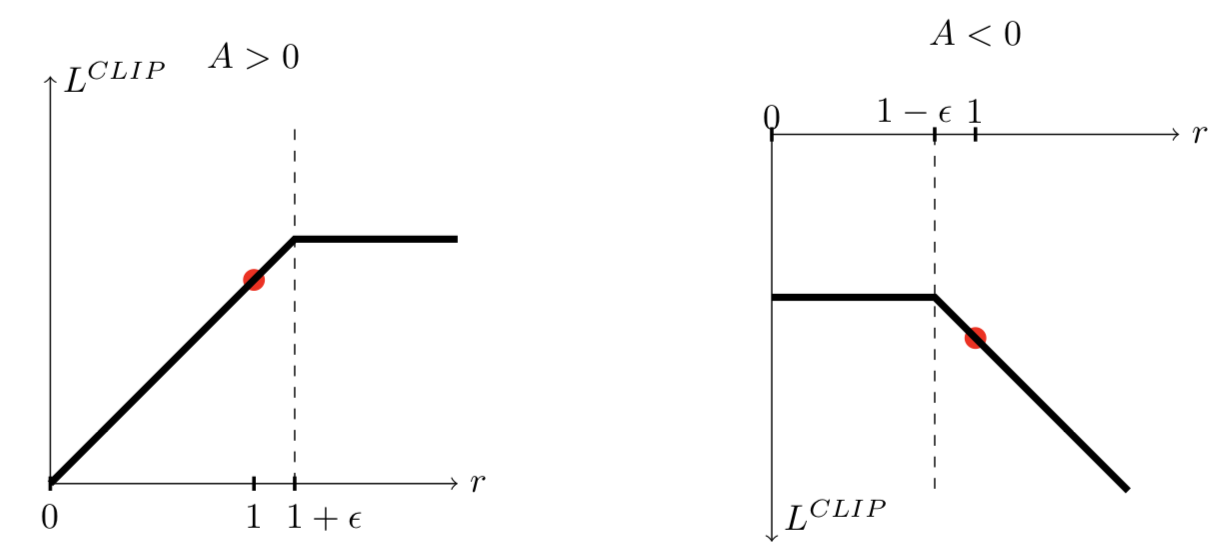
You will notice in the image below (taken from the PPO paper) that there are certain values of \(r_t(\theta)\) where the gradient is 0. When the advantage is positive, the cutoff point is \(1 + \epsilon\). When the advantage is negative, the cutoff point is \(1 - \epsilon\). By taking the minimum of the clipped and unclipped objective, as demonstrated below, we are creating a lower bound on the unclipped objective. In other words, we ignore a change in \(r_t(\theta)\) when it makes the objective improve, which is why the lower bound is also known as the pessimistic bound.
Our implementation has a unique feature that I haven’t mentioned yet: after the convolutional layers, we concatenate a series of one hot encodings that correspond to previous actions that our agent took. The reason we do this is because there are a few cases in which a combination of buttons need to be pressed in a sequential order. By taking previous actions into account, we allow our agent to learn such sequences. The video shown below was created after relatively little training using PPO on a Macbook Pro. I plan on running the algorithm for longer and updating the video sometime in the near future:
Concluding Remarks
In this post, we covered a lot of reinforcement learning background and learned how PPO works. We see that using GAE with PPO is a clever way to deal with the credit assignment problem, while keeping bias in check. We also learned a little bit about convolutional neural networks as a way to deal with pixelated inputs. I hope you can take what you learned in this post and apply it to your favorite games!